Machine integration
We connect the motion mechanisms, sensors, pneumatics, safety circuits and measuring instruments into a machine that runs the whole process by itself, with every interface clearly defined.
Industrial Automation
Conveyors and pneumatic motions on an ordinary production line are done quickly and cheaply by control panel builders. We take on a different kind of job: the kind where whether the mechanism moves accurately directly decides whether the measurement is right. From servo and BLDC motor control and multi-axis synchronization to waveband and camera selection for vision inspection stations, we plan the whole station together.
The goal is simple: turn a measurement that used to be set up and judged by hand into a station on the line that runs at the push of a button, with traceable results.
We connect the motion mechanisms, sensors, pneumatics, safety circuits and measuring instruments into a machine that runs the whole process by itself, with every interface clearly defined.
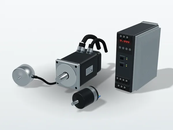
Selection, tuning and multi-axis synchronization of AC servo and BLDC motors, with drive firmware developed as well where needed. This part is expanded in section 2 below.
Operator interface, recipe management, and automatic recording and traceability of measurement data, so the station runs without an engineer standing beside it.
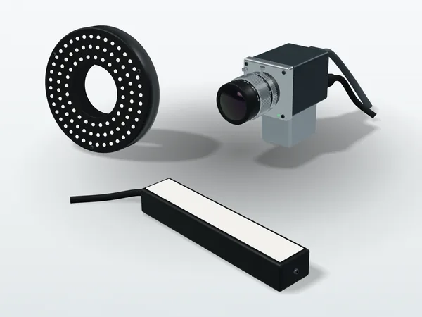
Waveband and camera selection from visible to LWIR, lens and lighting configuration, and converting "what defect needs to be seen" into resolution, depth of field and exposure conditions. This part is expanded in section 3 below.
The biggest difference between a measurement station and an ordinary production mechanism is that "moving fast" is not the point; "stopping steadily, stopping accurately, and knowing where it stopped" is. Below are the decisions we go through on every project.
The difference is not just price. Choose wrong, and no amount of tuning later will make up for it.
| Comparison | AC servo motor | BLDC motor |
|---|---|---|
| Feedback | Closed loop with an encoder; absolute encoders know the position at power-up, incremental ones must home first | Hall sensors or an encoder; sensorless commutation in some applications |
| Best suited to | Point-to-point positioning and contouring, where stiffness and repeatability are needed | Continuous rotation, low cost, and direct drive where space is limited |
| Typical place in an optoelectronic system | XY stages, Z-axis focusing, rotary indexing tables | Gimbal elevation and azimuth, scanning mirrors, filter wheels |
| Drive | Usually an off-the-shelf servo drive; the focus is on parameter tuning | Drive electronics and commutation firmware often have to be developed in-house |
| Most common pitfall | An inertia ratio too high to raise the gain, leading to long settling times | Uneven commutation at low speed, creeping caused by cogging, winding temperature rise |
The first thing to calculate in selection is the inertia ratio. The load inertia referred to the motor shaft, divided by the motor's own rotor inertia, is generally recommended to stay within 10:1; for measurement stages that need high response and short settling time, it is best kept to 5:1 or even 3:1. In a system with too high an inertia ratio, raising the gain causes oscillation and lowering it makes the axis soft, and nothing you tune is right. At that point what needs to change is the gear ratio or the motor, not more parameter tuning.
A servo system is not one loop but three nested loops. Without understanding this structure, tuning is just trial and error.
The standard tuning order is from the inside out:
If halfway through you find that "the velocity loop oscillates however it is tuned", the answer is usually not in the parameters but in the mechanism: a coupling that is not stiff enough, a belt that is too long, an under-supported lead screw, or the inertia ratio mentioned above.
However well the three loops above are tuned, they can only be as accurate as the feedback tells them. Common principles for angle feedback also include inductive encoders and resolvers; here we compare the three that are most often traded off against each other: optical, magnetic and capacitive. The differences between them are usually not in the resolution figures in the catalog, but in what each of them is vulnerable to, and that is often exactly what your site happens to have.
| Principle | How it measures | Strengths | Watch out for |
|---|---|---|---|
| Optical | Light passes through (or reflects from) a graduated grating, and photodetectors read the changes in light and dark | High-end products reach very high resolution and accuracy; the traditional choice for precision measurement | Dust, oil and condensation block the light path directly; the light source has a finite life; more sensitive to mounting eccentricity and temperature changes |
| Magnetic | Reads the direction of the magnetic field of a magnetized rotor | Resistant to contamination and vibration, simple construction, low cost; sealed versions reach high protection ratings | It works right next to the motor, so stray fields from the permanent magnets and drive currents can interfere, requiring shielding or a design that rejects external fields; accuracy is usually more conservative than high-end optical |
| Capacitive (electric field) | The rotor changes the capacitance distribution between the stator's transmitting and receiving electrodes, and the angle is solved from it | Not affected by magnetic fields; no light source, so no light source life limit; can be made as a very thin hollow ring | Conductive contamination and condensation affect the measurement; most products have a modest protection rating on their own and rely on the mechanical housing for protection |
So once the accuracy requirement is settled, selection usually comes down to three things: how strong the nearby magnetic field is (with a direct-drive motor right next to it, a magnetic solution needs extra handling of stray fields, which often makes it uneconomical), the contamination and condensation conditions on site, and how much space and weight the mechanism has left. Once these three questions are answered, the options usually narrow down.
For the capacitive column, the brand we often use is Netzer Precision. The reasons for choosing it fall into two groups: one comes from its mechanical form, the other from the measuring principle and product design. Looking at them separately makes it clearer which are choices of this brand and which are properties shared by the capacitive principle.
From the mechanical form: the sensing ring is hollow and thin, and has no bearing of its own. The rotor is fixed directly to the measured shaft and the stator to the frame, with no contact between them. This kit-type, bearingless form is not unique to capacitive encoders; optical and magnetic encoders also come in similar forms. The following benefits come from this mechanical form itself:
From the measuring principle and product design: it measures an electric field, not a magnetic field and not light.
It is not a universal answer either. In environments with coolant spray or condensation, conductive contamination directly affects capacitive measurement, and the products themselves mostly have modest protection ratings that the mechanical housing has to make up for; for linear measurement needing extremely high resolution, an optical scale is still the more direct choice.
A UAV gimbal is a case where all of these properties are used at once: the hollow shaft lets video and power cables run through the center of the axis, the bearingless form reduces the overhung mass of two- or three-axis gimbals, absolute output lets the gimbal know where it is pointing as soon as it is powered up, and immunity to magnetic fields matters because the magnets of the BLDC direct-drive motor are only a few centimeters away. How the gimbal's counterweighting, inertia and pointing error go into the same budget is covered in the gimbal section of the UAV EO/IR payload page.
A final reminder about the easiest thing to get wrong: resolution is not accuracy. An encoder that can resolve 0.001° does not mean the mechanism stops to within 0.001°; the whole transmission chain and thermal drift lie in between. The full breakdown is in How to Choose a Servo Motor: Three Numbers That Decide Whether a Mechanism Moves Accurately.
Many people assume that shortening the cycle time means turning up the speed. For a measurement station, what really eats the time is often the part after arrival, "waiting for it to stop vibrating".
So when we plan cycle time, we do not measure "whether the command says it has arrived", but the time from the in-position signal to the mechanism actually coming to rest within tolerance. This time can be measured with an accelerometer, or by shooting a burst with the measurement camera itself and seeing when the image stops changing; the latter is closer to the real acceptance condition.
When a measurement station has to shoot on the move (on-the-fly capture), the timing between motion and image capture becomes part of the accuracy.
There are two layers to the solution. The first is triggering by position rather than by time: the position compare output of a motion control card compares encoder counts directly and sends a pulse when the set position is reached, without going through the operating system, so jitter can be kept below a microsecond. The second is synchronizing the whole chain: EtherCAT distributed clocks give all nodes a common time base, typical control cycles are between 250 µs and 1 ms, and synchronization jitter between nodes can be kept within 1 µs; CANopen (with the CiA 402 drive profile) suits applications with few axes and less extreme real-time requirements.
If site conditions allow stop-and-shoot, stop and shoot: it is the simplest and most stable approach. On-the-fly capture is a measure for when the cycle time really cannot be brought down otherwise, and both of the points above have to be done along with it.
In most cases an off-the-shelf drive is fine. Only in the following situations, where off-the-shelf products often do not fit, is in-house development worth considering:
Our usual split is: the FPGA handles encoder decoding, PWM generation and hardware-level synchronized triggering, the work that needs deterministic timing; the MCU runs the velocity and position loops, communication protocols and the state machine; the current loop goes in the FPGA or in the highest-priority interrupt of the MCU, depending on the bandwidth needed. The benefit of splitting it this way is that timing-sensitive parts are not affected by software scheduling jitter.
This table is compiled from situations that really occur. The symptoms all look like "not accurate enough", but the causes lie at completely different levels.
| Symptom on site | Common causes | Where to start checking |
|---|---|---|
| The in-position signal is out, but the image is blurred | Settling time too short; the mechanism is still vibrating | Switch to an S-curve profile; measure the time between the in-position signal and actual rest |
| Stop-start jerking at low speed (creeping) | Static friction, cogging torque, insufficient current loop gain | Commutation angle calibration, current loop tuning, lubrication and preload checks |
| Multi-axis interpolation comes out as a staircase | Axis commands not synchronized, bus cycle too long | Switch to distributed clocks, shorten the control cycle, check each axis's feedforward settings |
| Image positions offset during on-the-fly capture (the same for the whole batch, or different for each image) | Trigger jitter, or time triggering used instead of position triggering | Switch to position compare output; measure the consistency of the delay from trigger to start of exposure |
| Accuracy drifts after an hour of warm-up | Thermal expansion of the structure, motor and drive temperature rise, heating of optical components | Establish a warm-up procedure, add temperature compensation, review materials and layout |
| Repeatability good at some times and poor at others | Backlash, loose couplings, poor repeatability of the home sensor | Home repeatability test, bidirectional repeatability test, mechanical inspection |
"What needs to be seen" decides the waveband, "how large the defect is" decides the resolution, and "how fast the line runs" decides exposure and lighting. Do it in the reverse order, and the most common result is buying a camera that cannot see the defect.
"Invisible defects" have completely different causes in different wavebands. First establish whether you are using reflection, transmission or the object's own emission; only then can you talk about cameras.
| Band | Wavelength | Why it can be seen | Typical tasks on the line |
|---|---|---|---|
| Visible / NIR | 0.4 – 1.0 µm | Reflected light, received directly by silicon sensors | Dimensional measurement, character and barcode reading, surface scratches and soiling |
| SWIR | 0.9 – 1.7 µm | Silicon becomes semi-transparent above 1.1 µm; water has an absorption band near 1.45 µm | Internal cracks in wafers and packages, moisture content, seeing contents through some plastics |
| MWIR | 3 – 5 µm | Objects at several hundred °C have their emission peak in this band; hydrocarbons have a characteristic absorption near 3.3 µm | High-temperature process monitoring, gas leak imaging |
| LWIR | 8 – 14 µm | Objects at room temperature (300 K) peak at about 9.7 µm, with no illumination needed | Abnormal temperature rise in motors, bearings and switchboards; thermographic non-destructive testing |
Assume a 100 mm wide field of view and a 2448 × 2048 camera (about 5 megapixels) with a 3.45 µm pixel pitch:
m = sensor width 8.45 mm ÷ field of view 100 mm = 0.0845How to calculate the focal length itself (working back from field of view and working distance) is covered in How to Calculate Lens Focal Length from Field of View and Working Distance. Next, the aperture decides the depth of field, but the same aperture also decides the diffraction limit, and the two pull in opposite directions:
| Aperture | Depth of field (approx.) | Airy disk diameter | Equivalent pixels |
|---|---|---|---|
| F/2.8 | 5.9 mm | 3.8 µm | 1.1 |
| F/5.6 | 11.7 mm | 7.5 µm | 2.2 |
| F/8 | 16.8 mm | 10.7 µm | 3.1 |
| F/11 | 23.1 mm | 14.8 µm | 4.3 |
At F/11, the blur from diffraction (4.3 px) is already about as large as the defect to be detected (4.9 px): the depth of field gained by stopping down eats the resolution it was meant to protect. A sensible operating point for this station is around F/5.6: about 12 mm of depth of field, with diffraction blur of about two pixels. If the height variation of the part exceeds this range, what needs solving is the fixture (bringing the measured surfaces back to the same height) or focusing and capturing in several passes, not stopping down further. A telecentric lens keeps magnification constant with height, which matters for dimensional measurement, but its depth of field is still limited by aperture and diffraction.
With the same camera and the same lens, changing the lighting method can turn "invisible" into "obvious at a glance". The four basic methods each correspond to a different type of defect:
With the wrong lighting method, no algorithm downstream can make up for it, because the contrast never made it into the image in the first place. The four lighting methods above apply to visible, NIR and SWIR (with light sources and filters changed to the matching band); thermal infrared (MWIR and LWIR) sees the radiation the object emits itself and needs no external lighting, and the radiation of objects at room temperature falls mainly in the LWIR.
If the part is moving, it travels some distance during the exposure and the image blurs. The amount of blur is simply speed times exposure time. Using the 40.8 µm pixel size from above, to keep blur within one pixel:
An exposure of only two hundred microseconds means there must be enough light within two hundred microseconds, which usually means strobed lighting rather than constant lighting. The other option is to stop the mechanism before shooting, at a cost that shows up directly in the cycle time (see the next section). In addition, use a global shutter wherever things move: a rolling shutter reads out line by line, so moving objects are captured skewed; if only a rolling shutter is available, the strobe must fall within the window when all rows are exposing at the same time.
Error in the trigger timing itself also becomes position error; that part was already calculated in 2.5 Synchronizing motion and image capture.
The cycle time of a measurement station is the sum of five segments. Laid out side by side, they usually show that the camera is not what needs to change.
Taking the station above as the example: the stage moves 50 mm into position (with the S-curve profile from section 2.4), a 5-megapixel camera, GigE transfer.
This chart makes just one point: to cut cycle time, first look at where the time goes. On this station, replacing the camera with one twice as fast saves less than 5 % of the total. The truly effective measures, in order, are:
Every one of these has a cost. Whether it is worth it depends on how many parts the line makes a day, which is a question we always ask at the requirements stage.
Turning parts that can each move on their own into a machine that runs the whole process by itself.
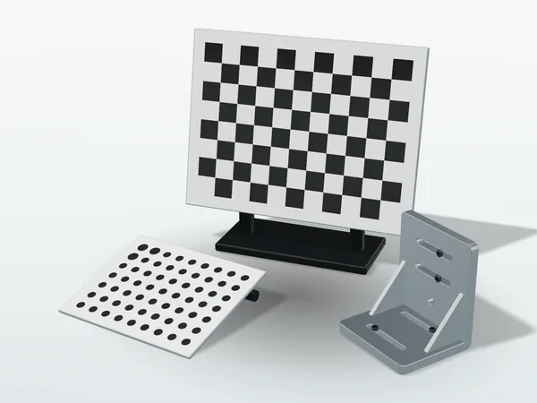
This work covers interface definitions between motion mechanisms and measuring instruments, sensor and I/O configuration, timing of pneumatic and fixture actions, safety circuits and emergency stop logic, and state machine design for loading, unloading and process flow. In most integration projects the difficulty is not in any single component but in making "who waits for whom" explicit: image capture waits for the mechanism to come to rest, the mechanism waits for the fixture to clamp, the fixture waits for the part to arrive. If any step lacks a clear completion signal, the whole machine can only wait on fixed delays, and the cycle time will not come down.
At delivery we also provide interface documents and timing diagrams, so whoever maintains the machine later does not have to reverse-engineer the program to know what it is waiting for.
A machine that moves is only the first step. Whether the site can operate it on its own, and whether results can be traced afterwards, decides whether it has really gone into production.
The key to interface design is that operators see only what they need: select a recipe, load the part, press start, read the result. Engineering mode and parameter adjustment sit behind access rights. Measurement results are saved automatically with time, recipe, machine status and operator, and where needed can be connected to an existing MES or database, so a quality issue can be traced back to the batch, the machine and the parameter set.
Turning "the direction a customer describes into performance tests that can be measured" is already one of our services; at the automation stage, those tests become the pass/fail conditions and report fields in the GUI.
The choice depends on real-time requirements and the customer's maintenance conditions; no one platform is always better.
An industrial PC with a motion control card. Suited to measurement stations where image acquisition, image processing and motion need to be tied together on the same machine; position compare output also lives at this level.
Multi-axis synchronization and distributed I/O. EtherCAT is used where there are many axes and distributed clock synchronization is required; CANopen suits mechanisms with few axes and simple wiring. EtherCAT, CANopen and pulse command are compared in EtherCAT and Multi-Axis Synchronization: Why Distributed Clocks Matter.
The solution when off-the-shelf drives cannot do the job. The FPGA handles encoder decoding, PWM and hardware synchronization, while the MCU runs the control loops and communication.
Each stage has an output you can accept. You can commission just one stage, or hand us the whole run.
| Stage | What is done | Deliverables |
|---|---|---|
| 01 Requirements and feasibility | Clarify the part, the defect definition and the cycle time and accuracy targets, and judge whether the job can be done | Requirement specification and feasibility assessment (including cases where it cannot be done, and why) |
| 02 Selection and optical validation | Waveband, camera, lens and lighting selection; shoot real samples to confirm the defect can really be seen | Selection list, sample images and interpretation results |
| 03 Mechanical and control design | Motion mechanism and axis layout, choice of control platform, interface and timing definitions | Mechanical drawings, interface documents, timing diagrams |
| 04 Integration and tuning | Assembly, servo tuning, boresight and coordinate calibration, measured cycle time | Tuning records, measured cycle time data |
| 05 Acceptance and handover | Acceptance item by item against the previously defined tests, plus on-site operation and maintenance instruction | Acceptance report, operation and maintenance instructions |
Stage 02 is deliberately placed before mechanical design. "Can this defect be seen in this waveband under this lighting?" is the highest-risk question in the whole project, and the time spent shooting samples is far cheaper than discovering after the mechanism is built that the defect cannot be seen.
Being clear about scope is more useful than promising everything.
It depends on how the station is made up. For a "stop, then shoot" measurement station like the example on this page, the comfortable range is about 300 to 800 ms per part. Getting below 100 ms usually takes three things at once: switching to capture on the move (position triggering), changing the transfer to CoaXPress or 10 GigE, and moving processing to an FPGA. Going further down to the 20 ms class is mostly the territory of line-scan cameras with dedicated lighting, where the mechanical and optical design approach is entirely different.
It is limited by the field of view and the sensor's pixel count, not by the algorithm. A defect must cover at least 3 to 5 pixels for a stable decision. With 5 megapixels and a 100 mm field of view (about 41 µm per pixel), the lower limit is about 0.12 to 0.2 mm. Going smaller means narrowing the field of view (shooting the same part at several positions, which lengthens the cycle time) or a camera with more pixels. This trade-off has to be decided at the requirements stage, not after the mechanism is built.
That is a lighting problem, not a camera problem. Mirror-like surfaces are usually handled with coaxial light or a diffuse dome; transparent parts often rely on backlight to measure the outline, or switch to SWIR to see inside directly. For this kind of project we recommend shooting samples before discussing specifications: quoting a specification without having shot anything is not good for either side.
An LWIR camera measures radiation, and converting it to temperature requires knowing the surface emissivity. When emissivity is unknown or changes (oxidation, oil, changing viewing angle), absolute temperature error can range from a few °C to several tens of °C: on a painted surface, an emissivity error of 0.1 gives about 2 to 5 °C (object at 50–80 °C, background at 25 °C), and on bare or semi-bright metal parts it can reach several tens of °C. But as long as the surface condition is consistent within a batch, relative differences between parts in the same batch are usually still reliable, which is why thermographic inspection on production lines relies mostly on relative judgment: not "this bearing is at 68 °C", but "this one is 12 °C hotter than the others in the batch". When absolute temperature is needed, a reference body of known emissivity has to be placed in the field of view.
When volumes are low, every part is different, or the defect cannot be clearly defined. The value of automation comes from repetition: for an inspection done only thirty times a year, manual work plus a fixture is usually more economical. An unclear defect definition is a more fundamental problem: if three experienced inspectors disagree about the same part, a machine will not have the answer either, and the first step is to write down the judgment criteria.
Items related to this page that we also supply, each with specifications and selection notes.
Original illustration, not a product photo. Actual appearance varies by model.
Write to us about what you need to measure, how you do it now, and the cycle time and accuracy you expect. Even if the conclusion is that "this should not be automated", we will explain why clearly.